Miles Shang home about

I’m working on a game that features a 2D starfield background that the user can pan and zoom. Here’s an interactive demo for the starfield component, which you can also find on github:

Controls: Click and drag to pan. Scroll or pinch to zoom.

Features

Pan and zoom limited only by floating point range and precision.
Time and space complexity independent of pan and zoom.
The entire map is mathematically pre-determined. You can revisit any spot and it will always look the same.
Not pre-generated. Only the area around the current viewport is generated at any given time.

How does it work?

The generator is derived from the construction of the Weierstrass function. First, the world is discretized by depth. At each depth interval, the world is further discretized in the $x$ and $y$ directions into tiles, with granularity determined by the level of depth. Using this method, we can assign an index to each tile and place a star in that tile with its position determined by hashing the index. Each star’s brightness is determined by its level of depth.

Mathematical principles

Suppose we had a function mapping each point in the plane to a value that represents the brightness of the nearest star at that point. To generate a visual representation of the starfield, we would evaluate this function at grid points corresponding to pixels in our viewport. If we could come up with such a function, what would it look like?

In order to look like a real starfield, the function should look random and bumpy. The night sky is mostly black with isolated points of light (stars) that are seemingly randomly spread out.
Like the night sky, the function should look roughly similar no matter how much you zoom in or pan around. In other words, it should be a fractal.
There should be a form of continuity. Zooming and panning by small amounts should produce only incremental changes in the output. It should not completely shuffle the whole view.

In order for a function to satisfy the first two conditions, it must be nowhere differentiable. Why? To be differentiable means that if you zoom in enough, you get closer and closer to a straight line. We want our function to be bumpy no matter how much you zoom in.

Weierstrass function

Given the requirements, we should start by looking into functions that are continuous and nowhere differentiable. One of the best known examples is the Weierstrass function, which is given as:

$W(x) = \sum_{n=0}^{\infty} a^n \cos(b^n \pi x)$

where $0 < a < 1$, $b$ is a positive integer, and

$a b > 1 + \frac{3}{2} \pi$

This function is the pointwise sum of infinitely many sine waves. As $n$ goes to infinity, the amplitudes and periods of these sine waves tend to zero by a geometric progression. Therefore, the summands look something like this:

n = (0:9)';
x = linspace(0, 2 * pi, 200);
y = diag((1/2) .^ n) * sin(2 .^ n * x);
plot(x, y);

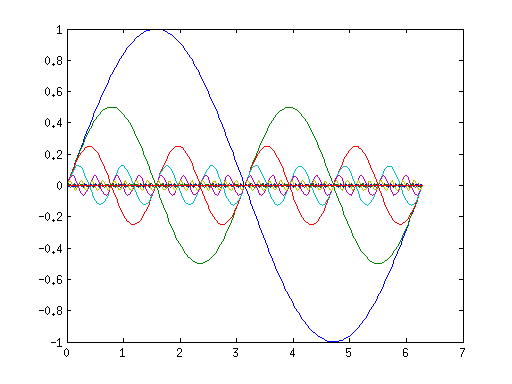
Sine waves with geometrically decreasing period and amplitude

Because the amplitudes rapidly decay to zero, we can trim the series after only a few terms as further terms won’t make a visible contribution at this zoom scale.

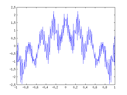
The end result looks like this:

a = 0.7; b = 8; n = (0:9)';
x = linspace(-1, 1, 200);
y = sum(diag(a .^ n) * cos(b .^ n * x * pi));
plot(x, y);

Weierstrass function - Wikipedia version

Zooming in:

a = 0.7; b = 8; n = (0:9)';
x = linspace(-0.1, 0.1, 200);
y = sum(diag(a .^ n) * cos(b .^ n * x * pi));
plot(x, y);

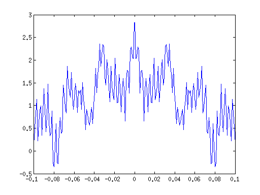
Weierstrass function - Wikipedia version - Zoomed

The Weierstrass function has the fractal property that we want, but it also has noticeable patterns that we don’t want. In fact, there’s nothing random about this function at all. Another problem is that if you zoom out enough, you’ll see that it doesn’t remain self-similar beyond a certain scale corresponding to the $n = 0$ starting point of the series.

To address these issues, Berry and Lewis (1980) extended the Weierstrass function into this complex-valued family of functions:

$W^\prime(t) = \sum_{n=-\infty}^{\infty} \frac{(1-e^{i\gamma^{n}t})e^{i\phi_n}}{\gamma^{(2-D)n}}$

where $1 < D < 2$, $\gamma > 1$, and $\phi_n$ is an arbitrary sequence of phases. By generating the $\phi_n$ pseudorandomly, we can inject some noise into the function. Here’s what that looks like:

rng(0);
gamma = 2; D = 1.9; n = (-10:10)';
phi = exp(i * rand(size(n)) * 2 * pi);
x = linspace(-1, 1, 200);
y = real(sum(diag(gamma .^ (-n * (2 - D))) * diag(phi) * (1 - exp(i * (gamma .^ n) * x))));
plot(x, y);

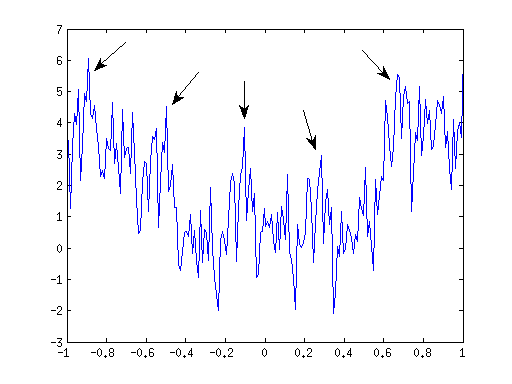
Weierstrass function - Berry and Lewis

Though it looks more random, there are still some latent patterns which you can see from the regular placement of the highest peaks (indicated by arrows). It seems like it’s not enough to add noise to the phases, we also need to alter the shapes of the components themselves.

So far we have only looked at functions of a single variable, but what we actually want is a function on the plane. Ausloos and Berman (1985) extended the Weierstrass function to multiple variables by adding up several copies of it, each turned by some angle and extruded to form a surface. In the simplest case:

$W_2 (x, y) = W'(x) + W'(y)$

where the $W’$ are defined as before, and each can have its own sequence of phases $\phi_n$.

This is roughly a sum of two-dimensional sinusoids like these:

[X, Y] = meshgrid(linspace(-pi, pi, 49), linspace(-pi, pi, 50));

for n = 0:3
    subplot(2, 2, n+1);
    Z = (1/2) ^ n * (cos(2^n * X) + cos(2^n * Y));
    surf(X, Y, Z); axis equal;
end

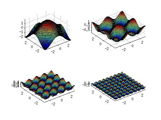
2D sine waves with geometrically decreasing period and amplitude

The end result looks like this:

rng(0);
gamma = 2; D = 1.9; n = (-10:10)';

x = linspace(-1, 1, 199);
phi = exp(i * rand(size(n)) * 2 * pi);
z1 = real(sum(diag(gamma .^ (-n * (2 - D))) * diag(phi) * (1 - exp(i * (gamma .^ n) * x))));

y = linspace(-1, 1, 200);
phi = exp(i * rand(size(n)) * 2 * pi);
z2 = real(sum(diag(gamma .^ (-n * (2 - D))) * diag(phi) * (1 - exp(i * (gamma .^ n) * y))));

surf(x, y, ones(size(y))' * z1 + z2' * ones(size(x)));

Weierstrass function - 2D

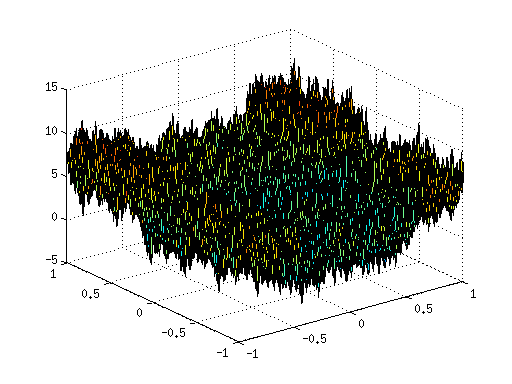
From here, it may be possible to produce a starfield using signal processing techniques. Though I did some research, I didn’t come up with anything that looks decent. Instead, we’ll use the same construction and adapt it to build a simulated point process.

Construction

A sine wave is a periodic function. It repeats the same shape over and over. For the $\text{sin}$ and $\text{cos}$ functions, that shape is a wave. What if, instead of a wave, we use a periodic function that is zero everywhere except at a single point? For example, consider the function $f(x) = [\text{cos}(x) = 1]$ where the square brackets $[~]$ are Iverson brackets. This function is $0$ everywhere except at $x = 0, -2\pi, 2\pi, -4\pi, 4\pi, \ldots$, where it takes the value $1$.

x = linspace(-10, 10, 200);
plot(x, cos(x)); hold on;
axis([-10, 10, -2, 2]); axis manual;
plot(x, ones(size(x)), '--g');
x = -2:2;
plot(2*pi*x, zeros(size(x)), 'Marker', 'o', 'MarkerEdgeColor', 'red', 'MarkerFaceColor', 'white', 'Color', 'red');
plot(2*pi*x, ones(size(x)), 'Marker', 'o', 'MarkerEdgeColor', 'red', 'MarkerFaceColor', 'red', 'LineStyle', 'none');
legend('y = cos(x)', 'y = 1', 'y = [cos(x) = 1]');

y = [cos(x) = 1]

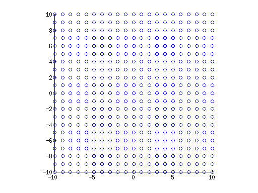
In two dimensions, a useful analogue is a function that places points in a grid pattern:

$f(x, y) = [\exists m, n \in \mathbb{Z}~\text{s.t.}~x = m~\text{and}~y = n]$

[X, Y] = meshgrid(-10:10, -10:10);
scatter(X(:), Y(:)); axis square;

Square grid

We also have analogues for period $p$ and amplitude $A$:

$f(x, y) = A [\exists m, n \in \mathbb{Z}~\text{s.t.}~x = mp~\text{and}~y = np]$

Create an infinite series of these functions. As with the Weierstrass function, set the period and amplitude to both be geometric sequences with respect to the index of summation.

$f(x, y) = \sum_{k=-\infty}^\infty a_A {r_A}^{k} [\exists m, n \in \mathbb{Z}~\text{s.t.}~x = a_p {r_p}^{k}m~\text{and}~y = a_p {r_p}^{k}n]$

For simplicity of implementation, choose $a_A = a_p = 1$ and $r_A = r_p = 1/e$.

$f(x, y) = \sum_{k=-\infty}^\infty e^{-k} [\exists m, n \in \mathbb{Z}~\text{s.t.}~x = e^{-k}m~\text{and}~y = e^{-k}n]$

In order to graph this function, we need a strategy for truncating the infinite series in relation to the current viewport scale. Start at an index that results in a tile size $p^2$ of approximately the same size as the viewport itself:

$k_{\min} = \max(k : e^{-2k} < w \cdot h) = \lfloor -\text{ln}(w \cdot h) / 2 \rfloor$

where $w$ is the width and $h$ is the height of the viewport.

On average, this term will place one star in the viewport and subsequent terms will place $e^2, e^4, \ldots$. Since we only need to see a constant number of stars at any given time, evaluate a constant number of terms of the series.

We also need to scale the amplitudes to fall between $0$ (completely dark) and $1$ (completely bright). The overall brightness of the visible stars should be zoom-invariant. In order to satisfy this property, divide the amplitudes by a scaling factor such that the amplitude of the $k_{\min}$ term is approximately constant. However, this scaling factor should vary continuously as you zoom, unlike the discrete indices of summation. Therefore, we consider $k_{\text{cont}} = -\text{ln}(w \cdot h) / 2$, which is $k_{min}$ without taking the floor function. Our scaling factor is the amplitude at $k_{\text{cont}}$.

$A_{k_{\text{cont}}} = \exp(\ln(w \cdot h) / 2) \\ A_{\text{rescaled}} = B A_k / A_{k_{\text{cont}}} = B \exp(-\ln(w \cdot h) / 2 - k)$

where $B$ is a brightness factor which allows us to control the overall brightness level.

Since the amplitudes fall off rapidly, we want to reshape the amplitude profile, pushing more of them towards $1$ while maintaining a smooth drop off. One quick way is to take the $\arctan$.

$A_{\text{reshaped}} = \frac{2}{\pi}\arctan(A_{\text{rescaled}})$

function getStars1(offsetX, offsetY, width, height) {
  var stars = [];
  var k_cont = -Math.log(width * height) / 2;
  var k_min = Math.floor(k_cont);
  for (var k = k_min; k < k_min + 5; k++) {
    var period = Math.exp(-k);
    for (var m = Math.floor(offsetX / period); m <= Math.ceil((offsetX + width) / period); m++)
      for (var n = Math.floor(offsetY / period); n <= Math.ceil((offsetY + height) / period); n++)
        stars.push(new Star(
          m * period,
          n * period,
          Math.atan(10 * Math.exp(k_cont - k)) * 2 / Math.PI));
  }
  return stars;
}

This is an interactive demo:

To get a random-looking starfield, we add some jitter to each star. We get a star’s jitter by hashing its index consisting of $k, m, n$ where $k$ is the index of summation for the term in the infinite series and $m, n$ are the tile’s index in the $x, y$ directions.

function getStars2(offsetX, offsetY, width, height) {
  var stars = [];
  var k_cont = -Math.log(width * height) / 2;
  var k_min = Math.floor(k_cont);
  for (var k = k_min; k < k_min + 5; k++) {
    var period = Math.exp(-k);
    for (var m = Math.floor(offsetX / period); m <= Math.ceil((offsetX + width) / period); m++)
      for (var n = Math.floor(offsetY / period); n <= Math.ceil((offsetY + height) / period); n++)
        stars.push(new Star(
          (m + hashFnv32a(k+':'+m+':'+n+':x') / (-1 >>> 1)) * period,
          (n + hashFnv32a(k+':'+m+':'+n+':y') / (-1 >>> 1)) * period,
          Math.atan(10 * Math.exp(k_cont - k)) * 2 / Math.PI));
  }
  return stars;
}

Tweaking

The final version of the starfield has a few more cosmetic tweaks.

In order to better approximate the look of true randomness, increase the range of the jitter so that stars can be placed far outside of their own tile.
Add jitter to the amplitudes for smoother zooming.
Further tweak the amplitudes by translating the $\arctan$ reshaping so that the faintest stars fade in more gradually.

References

Ausloos M, Berman DH. 1985. A Multivariate Weierstrass-Mandelbrot Function. Proc R Soc Lond A, 400:331-50
Berry MV, Lewis ZV. 1980. On the Weierstrass-Mandelbrot Fractal Function. Proc R Soc Lond A, 370:459-84